The Logic Behind AI Prediction in Sports Betting
AI sports prediction comes down to a five-stage pipeline: collect historical game data, clean it, engineer features, train a machine-learning model, and finally compare predicted win rates against live odds to surface positive-EV bets. Compared with relying on human intuition alone, machine learning lifts prediction accuracy by roughly 15% on average. This article uses the NBA as a worked example and breaks down the implementation logic of every step.
Want the backtest results first? The model’s real win rate and profit curve across 13,000+ games and 53 iterations are laid out on theAI Model Performance page.
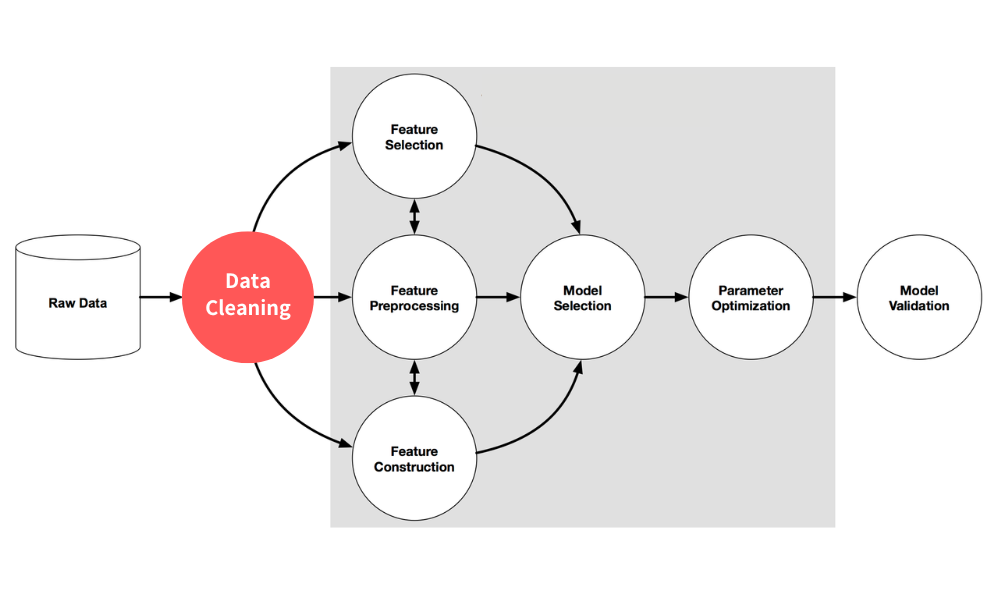
The Prediction Pipeline: Five Steps at a Glance
One Pipeline, Five Stages
From raw data to positive-EV bets — watch the data flow down the pipeline.
Collect Season Data
Pull 3 million-plus historical records from Basketball-Reference and stats.nba.com
Clean the Data
Handle missing values, duplicates and outliers, and standardize formats to guarantee data quality
Engineer Features
Extract the most predictive features — Elo Rating, recent form, injuries, PER and more
Train the Model
Backtest random forests, logistic regression and other models to find the highest test accuracy
Compare Odds for Value
Compute expected value by matching AI win rates against live odds, betting only positive-EV lines
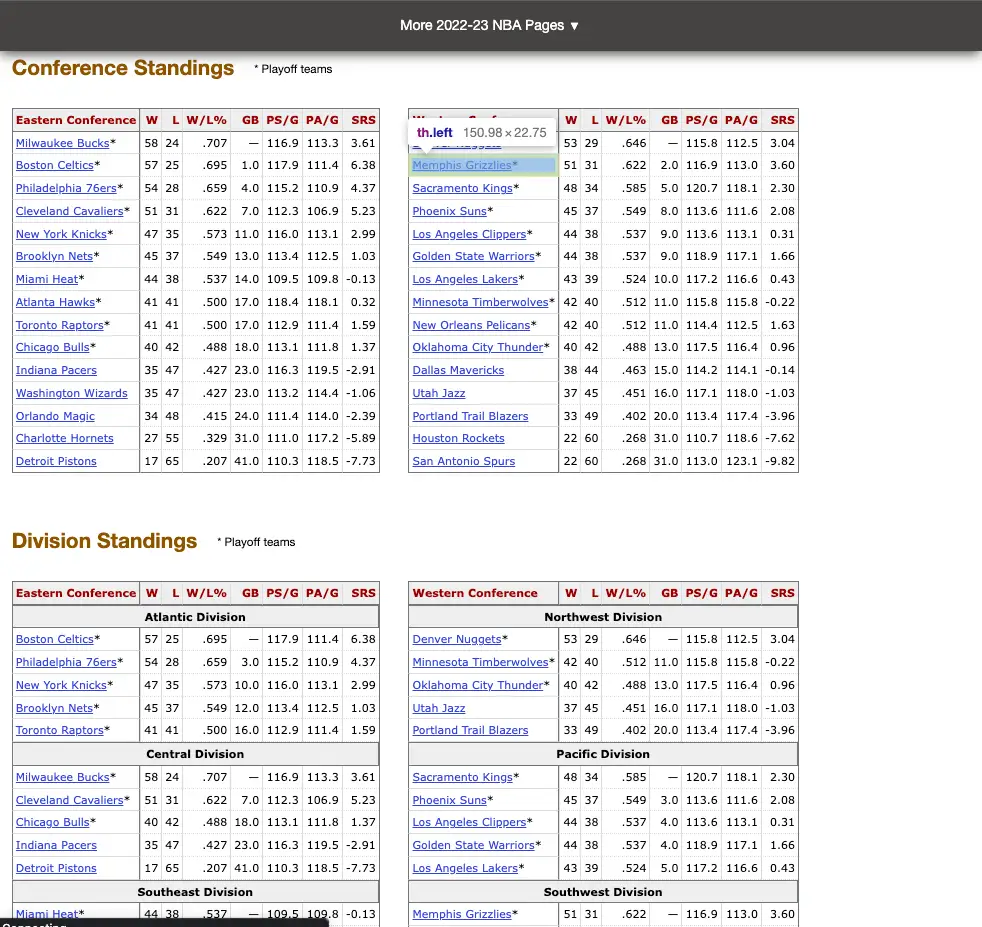
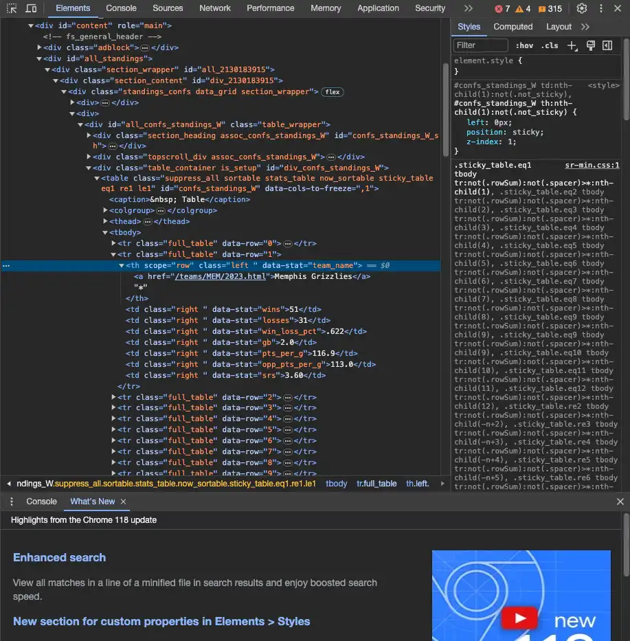
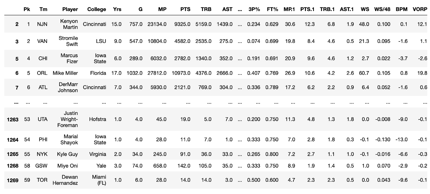
Scraping NBA Season Data
The data comes from Basketball-Reference and stats.nba.com, covering every game since 1946 — over 3 million team and player records: wins and losses, total points, rebounds, assists, turnovers, steals, three-point percentage, free-throw attempts and more. Both sources accept custom date ranges; technically, we read the HTML with Python’s requests, then parse out the tables we need using Pandas’ pd.read_html() or BeautifulSoup.
The raw columns are normalized first so that downstream cleaning and feature engineering share a consistent schema:
COLUMN_MAP = {
    'PName': 'Player_Name',      # player name
    'POS':   'Position',         # position
    'Team':  'Team_Abbreviation',
    'GP':    'Games_Played',
    'W':     'Wins',
    'L':     'Losses',
    'Min':   'Minutes_Played',
    'PTS':   'Total_Points',
    'FG%':   'Field_Goal_Percentage',
    '3P%':   'Three_Point_FG_Percentage',
    'FT%':   'Free_Throw_Percentage',
    'REB':   'Total_Rebounds',
    'AST':   'Assists',
    'TOV':   'Turnovers',
    'STL':   'Steals',
    'BLK':   'Blocks',
    # ... 29 columns in total, incl. OREB / DREB / PF / FP / DD2 / TD3
}
Data Cleaning
Data cleaning sets the ceiling on what the model can achieve. Raw data is riddled with input errors, missing values, duplicates and outliers that must be cleaned out first. Two easily overlooked points matter most: first, drop any column that leaks the final outcome so the model can’t cheat its way to the answer; second, remove highly correlated redundant features (field-goal, two-point and three-point percentages all overlap, for example) to reduce multicollinearity.
Handle Missing Data
Drop, sensibly impute, or model-estimate missing values so the training set has no holes.
Remove Duplicates
Detect and drop duplicate entries so every game and player record is unique.
Treat Outliers
Use statistical methods or algorithms to flag extreme values so a single blow-up game doesn’t skew the model.
Enforce Consistency
Standardize player-name spellings and reconcile formats across sources so all the data speaks one language.
Feature Engineering: Five Key Features
At its core, feature engineering turns each team’s ability into comparable numbers, surfacing the factors and weights that decide a game — ignoring team names and reputation, looking only at the hard numbers. In a deep-learning NBA implementation, the five features below carry the most predictive power for game outcomes.
Features Ranked by Predictive Power
Relativized team metrics (Elo) far outweigh individual player efficiency (PER) — the model’s most decisive trade-off.
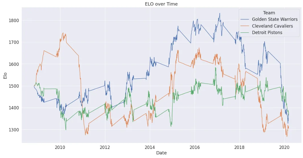
1. Elo Rating: Measuring Team Strength from Results
Elo Rating only needs each game’s final score, location and date to work. Wins add points, losses subtract them, and an upset or blowout win earns more; it is a zero-sum system, so the points one team gains the opponent loses. Every team usually starts at the median of 1500. The post-game update formula is:
Elo_new = Elo_old + K × (Result − WinProbability)

Elo_old        current Elo Rating
K              tuning parameter: the larger K is, the faster ratings move
Result         actual outcome (win = 1, loss = 0)
WinProbability predicted win rate derived from the two teams' Elo gap
Elo also carries across seasons — strong teams tend to stay strong and weak teams rarely flip overnight — so each new season starts by regressing the previous season’s final rating 25% toward the league average of 1505:
Elo_next_season = (R × 0.75) + (0.25 × 1505)

R = the team's final Elo rating from last season
Chart any three teams’ Elo over time and the season-long ebb and flow jumps out: in the year the Warriors and Cavaliers met in the Finals their Elo peaked together; the West being tougher overall than the East shows up as the extra Elo the Warriors banked from “quality wins”; and the roster losses and injuries after a title run send the curve sliding just as fast.
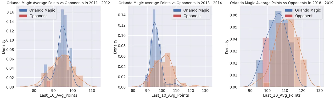
2. Recent Team Form (Last 10-Game Average)
Average each team’s last 10 games for points, rebounds, assists, turnovers, blocks and steals, and store them as new feature columns. The art is in feature selection: use correlation analysis, principal component analysis (PCA) and information gain to keep the most informative columns. To capture trend and seasonality on top of that, layer in time-series models (ARIMA, LSTM), or hand the features straight to an SVM, decision tree or random forest to learn the nonlinear relationships between them.
3. Recent Player Form (Last 10-Game Average)
Beyond the team level, each player’s recent form is a signal too. After pulling game-by-game detail from nba.com/stats, compute a last-10-game average for every player. Take two stars as an example:
| Player | PTS | REB | AST | TOV | BLK | STL |
|---|---|---|---|---|---|---|
| LeBron James | 28.5 | 7.8 | 7.2 | 2.3 | 1.1 | 1.5 |
| Stephen Curry | 31.2 | 5.6 | 6.8 | 2.1 | 0.3 | 1.7 |
Different players show their value in different columns (a scorer vs a rebounding center), and feature selection is again driven by correlation analysis, PCA and information gain.
4. Player Season Performance (Prior & Current Season)
Averages alone distort the picture — players get hurt and rotate in and out, so the model cares more about how each game deviates from a player’s own baseline. A complete assessment has to weigh five dimensions at once:
Average Box-Score Stats
Points, assists, rebounds, steals, blocks and turnovers — always read alongside position and scheme so surface numbers don’t mislead you.
Injury Status
The injured area and projected recovery time directly drive availability and post-return form swings — a critical model input.
Minutes Played
The minutes gap between starters and bench players inflates or compresses raw stats; big output in few minutes signals high efficiency.
Position & Playing Style
A shooting guard and a center carry different roles, and team scheme (ball movement vs isolation) reshapes the stat line.
Game Context
Coasting on a lead slows the pace and deflates stats while chasing a deficit inflates them — the win/loss context must be factored in.
5. Player Efficiency Rating (PER)
Just as Elo does for teams, Hollinger’s PER folds seemingly unrelated stats into a single index that “relativizes” player performance. NBA stat lines are easily inflated or compressed by minutes and matchup (bench vs starter), and PER fixes this with a per-minute normalization — weighting each offensive and defensive stat, then multiplying by the inverse of minutes played:
PER = ( FGM × 85.910  + STL  × 53.897 + 3PTM × 51.757
      + FTM × 46.845  + BLK  × 39.190 + OREB × 39.190
      + AST × 34.677  + DREB × 14.707 − PF   × 17.174
      − FT_Miss × 20.091 − FG_Miss × 39.190 − TOV × 53.897
      ) × (1 / Minutes)
Data Analysis & Model Training
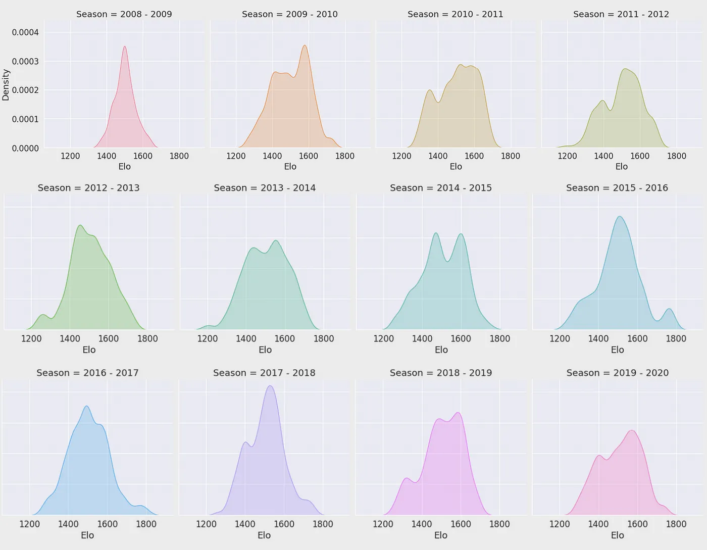
Two questions sit at the heart of the analysis: does Elo truly correlate with the other stats and line up correctly? And does predicting game outcomes work better with team stats (Elo) or player stats (PER)?
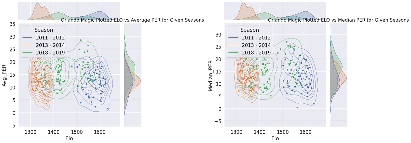
Start with the league-wide Elo distribution density each season: a near-normal shape means a balanced league, while a long tail means a “super-team” has emerged. Track a single team and the higher its average scoring the higher its Elo tends to be — yet at similar scoring levels Elo still varies widely; only once you make scoring relative to the opponent and to the league average does the correlation truly stabilize. That is the proof that Elo predicts outcomes better than raw points precisely because it is a relativized stat. PER tells the opposite story: line up a team’s PER sum, mean and median against the team strength Elo measures, and the correlation is weak across the board — high player efficiency doesn’t mean more points, and what actually decides a matchup (and in turn drives Elo) is relative scoring.
Two Core Takeaways
- Relativizing is what makes it stable: only once scoring is expressed relative to the opponent and the league does its correlation with outcomes truly hold.
- Team > sum of players: summed PER correlates weakly with team strength — high player efficiency does not mean the team wins.
Test Accuracy vs the Theoretical Ceiling
The best NBA prediction models top out near 70%; at 67.15% the random forest is already closing in — the remaining gains lie in model choice, not tuning.
When predicting outcomes from player scoring, we used linear regression (predicting a continuous score) rather than logistic regression (predicting only win/loss), then summed each team’s predicted points to compare. The 58.66% accuracy confirms the earlier observation: combined player performance is far too variable, nowhere near as consistent as team-level form. The best result — a random forest tuned with RandomizedSearchCV — reached a 67.15% peak test accuracy, and since even the strongest NBA prediction models cap out around 70%, the model is already closing in on the theoretical ceiling. From here, the payoff comes from investing time in model choice (SGD classifier, linear discriminant analysis, convolutional networks, naive Bayes) rather than endless tuning.
Odds Comparison: From Predicted Win Rate to Positive EV
A model’s win rate alone doesn’t make money; the profit formula needs three ingredients: the deep-learning predicted win rate, live odds, and a backtested staking strategy. Match the AI win rate against the market odds to compute expected value (EV), and only act when the EV is positive:
EV = (AI win rate × decimal odds) − 1

EV > 0  →  positive expected return over the long run (value bet)
EV < 0  →  a long-term loser, skip it

Example: AI win rate 58%, odds 1.90
EV = (0.58 × 1.90) − 1 = +0.102 → +10.2% expected per bet
This approach isn’t limited to the NBA — it applies to basketball, baseball, soccer, hockey and tennis alike. You can review the model’s hit rate and units won on real games month by month onAI Model Performance, and run quick pre-bet expected-value and parlay-odds calculations with theBetting Calculators.
One Framework, Covering the World’s Major Leagues
Because feature engineering is about comparing ability rather than reading team names, the same pipeline ports across sports: it currently covers the NBA, MLB, the top five soccer leagues, European competitions and the NHL, with more leagues to come.
 NBA
NBA MLB
MLB EPL
EPL La Liga
 Bundesliga
 Serie A
 Ligue 1
 UCL
UCL UEL
UEL MLS
MLS NHL
NHL
Conclusion & Next Steps
- Relativized stats beat raw numbers: Elo is more accurate than average points, and points beat summed PER, because winning is relative by nature.
- Team-level features are more stable than the sum of players and form the model’s primary signal; player form serves as a supporting feature.
- A 67.15% test accuracy already approaches the roughly 70% theoretical ceiling for NBA prediction; the remaining gains lie in model choice, not endless tuning.
- A predicted win rate only turns into long-term profit when paired with odds comparison and positive-EV discipline.
References & Data Sources
Every method and dataset in this article is publicly verifiable — feel free to dive into the original research:
Now That You Get the Algorithm, Run Your Own Bets on Data
Log every bet for free and automatically track your win rate, ROI and bankroll curve — so you can backtest your own staking strategy just like a model does.